TensorFLow 基础(1)

TensorFLow 基础(1)

hi,又和大家见面了,上一次我们讲了建立模型步骤和一些基础的概念(Tensor、Placeholder),那么我们这次就继续我们的矩阵操作,因为在TensorFlow处理一些数学问题的时候,往往都是通过矩阵来存储数据,通过特定的矩阵运算,我们实现数据的处理,从而得到一些数据的特性。还有一些其他的Tensorflow的概念,我希望大家能坚持下去,只要将这些基础的概念学会,那么以后运用TensorFlow就会得心应手。

  1. 和TensorFlow一起工作的Matrices
1
2
3
4
5
6
7
8
9
10
11
12
13
14
15
16
17
18
19
20
21
22
23
24
25
26
27
28
29
30
31
# 矩阵和矩阵操作
import tensorflow as tf
import numpy as np
from tensorflow.python.framework import ops
ops.reset_default_graph()
sess = tf.Session()
identity_matrix = tf.diag([1., 1., 1])
print(sess.run(identity_matrix)) #注意这个地方,如果是TensorFlow的Tensor,
# 那么使用sess的run方法才能将结果显示
# 或者下面这种方式
print(identity_matrix.eval(session = sess))
A = tf.truncated_normal([2, 3]) # 2 * 3 大小 均值0 方差为1.
print(sess.run(A))
B = tf.fill([2, 3], 5.) # 2 * 3 使用5.填充
print(sess.run(B))
C = tf.random_uniform([3, 2]) # 3 * 2 随机初始化
print(sess.run(C))
D = tf.convert_to_tensor(np.array([[1., 2., 3.], [-3., -7., -1.], [0., 5., -2.]]))
print(sess.run(D))

print(sess.run(A+B)) # 加法和 tf.add() 一样
print(sess.run(B-B)) # 减法和 tf.subtract() 一样
print(sess.run(tf.matmul(B, identity_matrix))) # 矩阵乘法
print(sess.run(tf.transpose(C))) # 矩阵转置
print(sess.run(tf.matrix_determinant(D))) # 计算行列式
print(sess.run(tf.matrix_inverse(D))) # 矩阵的逆
print(sess.run(tf.cholesky(identity_matrix))) # cholesk分解(平方根分解)

eigenvalues, eigenvectors = sess.run(tf.self_adjoint_eig(D)) # 求特征向量和特征值
print(eigenvalues)
print(eigenvectors)
  1. Math Operation(数学操作)
1
2
3
4
5
6
7
8
9
10
11
12
13
14
15
16
17
18
19
20
21
22
23
24
25
26
27
28
29
30
import matplotlib.pyplot as plt
import numpy as np
import tensorflow as tf
from tensorflow.python.framework import ops
ops.reset_default_graph()

sess = tf.Session()
# math operation
print(sess.run(tf.div(3, 4)))
print(sess.run(tf.truediv(3, 4)))
print(sess.run(tf.floordiv(3., 4.)))
print(sess.run(tf.mod(22., 5.)))
print(sess.run(tf.cross([1., 0., 0.], [0., 1., 0.])))
# Trig operation
print(sess.run(tf.sin(3.1416)))
print(sess.run(tf.cos(3.1416)))
print(sess.run(tf.div(tf.sin(3.1416 / 4.), tf.cos(3.1416 / 4.))))
# custom operation
# f(x) = 3 * x^2 - X + 10

test_nums = range(15) # 生成一个list
def custom_polynomial(x_val):
return (tf.subtract(3 * tf.square(x_val), x_val) + 10)
print(sess.run(custom_polynomial(11)))

# list expend
expected_output = [3 * x * x - x + 10 for x in test_nums]
print(expected_output)
for num in test_nums:
print(sess.run(custom_polynomial(num)))
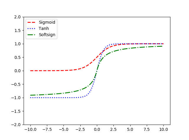
  1. Activation Function(激活函数)
1
2
3
4
5
6
7
8
9
10
11
12
13
14
15
16
17
18
19
20
21
22
23
24
25
26
27
28
29
30
31
32
33
34
35
36
37
38
39
40
41
42
43
44
45
# 激活函数主要是为了让神经网络模型具有非线性的特性
import matplotlib.pyplot as plt
import numpy as np
import tensorflow as tf
from tensorflow.python.framework import ops
ops.reset_default_graph()
sess = tf.Session()
x_vals = np.linspace(start = -10, stop = 10, num = 100)
# Relu Activation-> max(0, x)
print(sess.run(tf.nn.relu([-3., 3., 10.])))
y_relu = sess.run(tf.nn.relu(x_vals))
# Relu6 Activation-> min(max(x, 0), 6)
print(sess.run(tf.nn.relu6([-3., 3., 10.])))
y_relu6 = sess.run(tf.nn.relu6(x_vals))
# Sigmoidactivation-> 见公式1
print(sess.run(tf.nn.sigmoid([-1., 0., 1.])))
y_sigmoid = sess.run(tf.nn.sigmoid(x_vals))
# Hyper Tangent activation->见公式2
print(sess.run(tf.nn.tanh([-1., 0., 1.])))
y_tanh = sess.run(tf.nn.tanh(x_vals))
# softsign activation->见公式3
print(sess.run(tf.nn.softsign([-1., 0., 1.])))
y_softsign = sess.run(tf.nn.softsign(x_vals))
# softplus activation->见公式4
print(sess.run(tf.nn.softplus([-1., 0., 1.])))
y_softplus = sess.run(tf.nn.softplus(x_vals))
# Exponential linear activation->见公式5
print(sess.run(tf.nn.elu([-1., 0., 1.])))
y_elu = sess.run(tf.nn.elu(x_vals))

plt.plot(x_vals, y_softplus, 'r--', label='Softplus', linewidth=2)
plt.plot(x_vals, y_relu, 'b:', label='ReLU', linewidth=2)
plt.plot(x_vals, y_relu6, 'g-.', label='ReLU6', linewidth=2)
plt.plot(x_vals, y_elu, 'k-', label='ExpLU', linewidth=0.5)
plt.ylim([-1.5,7])
plt.legend(loc='upper left')
plt.show()

plt.plot(x_vals, y_sigmoid, 'r--', label='Sigmoid', linewidth=2)
plt.plot(x_vals, y_tanh, 'b:', label='Tanh', linewidth=2)
plt.plot(x_vals, y_softsign, 'g-.', label='Softsign', linewidth=2)
plt.ylim([-2,2])
plt.legend(loc='upper left')
plt.show()
下图给出激活函数的曲线图

公式1:

\[ \sigma(x)=\frac{1}{1+e^{-x}} \]

公式2:

\[ f(x)=\frac{e^x-e^{-x}}{e^x + e^{-x}} \]

公式3:

\[ f(x) = \frac{1}{1 + |x|} \]
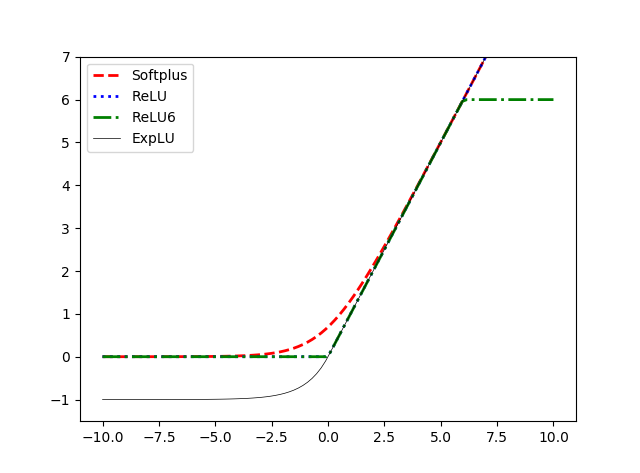
公式4

\[ f(x) = \log(1 + e^x) \]

公式5:

\[ elu(x) = \begin{cases} x & x > 0 \\ \alpha(exp(x) - 1) & x \leq 0 \end{cases} \]

-

-

  1. Operations on a Computational Graph
1
2
3
4
5
6
7
8
9
10
11
12
13
14
15
16
17
18
19
20
21
22
23
24
25
26
27
28
29
import os
import matplotlib.pyplot as plt
import numpy as np
import tensorflow as tf
from tensorflow.python.framework import ops
ops.reset_default_graph()

sess = tf.Session()

# 创建的数据是要喂给下面的placeholder的
x_vals = np.array([1., 3., 5., 7., 9.])

# 创建placeholder
x_data = tf.placeholder(tf.float32)

# 创建一个乘数
m = tf.constant(3.)

# 乘法
prod = tf.multiply(x_data, m)
for x_val in x_vals:
print(sess.run(prod, feed_dict = {x_data: x_val}))

#下面将数据计算图输出到文件里面,供我们后来启动tensorboard使用
merged = tf.summary.merge_all(key = 'summary')
if not os.path.exists('tensorboard_logs/'):
os.makedirs('tensorboard_logs/')

my_writer = tf.summary.FileWriter('./tensorboard_logs/', sess.graph)
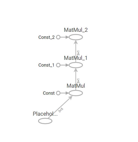
  1. Layering Nested Operations
1
2
3
4
5
6
7
8
9
10
11
12
13
14
15
16
17
18
19
20
21
22
23
24
25
26
27
28
29
30
31
32
33
34
35
36
37
38
39
40
41
42
import matplotlib.pyplot as plt
import numpy as np
import tensorflow as tf
import os
from tensorflow.python.framework import ops

ops.reset_default_graph()

sess = tf.Session()

# 创建数据为了feed
my_array = np.array([[1., 3., 5., 7., 9.],
[-2., 0., 2., 4., 6.],
[-6., -3., 0., 3., 6.]])

# 复制
x_vals = np.array([my_array, my_array + 1])

# 声明placeholder
x_data = tf.placeholder(tf.float32, shape = [3, 5])

# 声明常数来操作
m1 = tf.constant([[1.], [0.], [-1.], [2.], [4]])
m2 = tf.constant([[2.]])
a1 = tf.constant([[10.]])

# 声明操作
prod1 = tf.matmul(x_data, m1)
prod2 = tf.matmul(prod1, m2)
add1 = tf.matmul(prod2, a1)

# 打印验证结果
for x_val in x_vals:
print(sess.run(add1, feed_dict = {x_data: x_val}))


#下面将数据计算图输出到文件里面,供我们后来启动tensorboard使用
merged = tf.summary.merge_all(key = 'summaries')
if not os.path.exists('tensorboard_logs/'):
os.makedirs('tensorflow_logs/')
my_writer = tf.summary.FileWriter('tensorboard_logs/', sess.graph)
#下图就是在操作过程中,tensorflow建立的图运算模型

-

  1. Working With Multiple Layers
1
2
3
4
5
6
7
8
9
10
11
12
13
14
15
16
17
18
19
20
21
22
23
24
25
26
27
28
29
30
31
32
33
34
35
36
37
38
39
40
41
42
43
44
45
import matplotlib.pyplot as plt
import numpy as np
import tensorflow as tf
import os
from tensorflow.python.framework import ops

ops.reset_default_graph()

sess = tf.Session()

x_shape = [1, 4, 4, 1]
# 定义一个4 * 4 大小的随机矩阵
x_val = np.randim.uniform(size = x_shape)

x_data = tf.placeholder(tf.float32, shape = x_shape)

# 定义一个空间移动窗口,也就是卷积操作的卷积核
# 大小是2 * 2, 步长是 2
# filter的值是一个固定的值0.25
my_filter = tf.constant(0.25, shape = [1, 2, 2, 1])
my_strides = [1, 2, 2, 1]
mov_avg_layer = tf.nn.conv2d(x_data, my_filter, my_strides, padding = 'SAME', name = 'Moving_Avg_Window')

# 第二层
def custom_layer(input_matrix):
input_matrix_sqeezed = tf.squeeze(input_matrix)
A = tf.constant([1., 2.], [-1., 3.])
b = tf.constant(1., shape = [2, 2])
output = tf.add(tf.matmul(A, input_matrix_sqeezed), b)
return tf.nn.relu(output)
with tf.name_scope('custom_layer') as scope:
custom_layer1 = custom_layer(mov_avg_layer)

# 运行结果
print(sess.run(mov_avg_layer, feed_dict = {x_data: x_val}))

print(sess.run(custom_layer1, feed_dict = {x_data: x_val}))

#下面将数据计算图输出到文件里面,供我们后来启动tensorboard使用
merged = tf.summary.merge_all(key = 'summaries')

if not os.path.exists('tensorboard_logs/'):
os.makedirs('tensorboard_logs/')
my_writer = tf.summary.FileWriter('tensorboard_logs', sess.graph)
# 下图是计算图

-

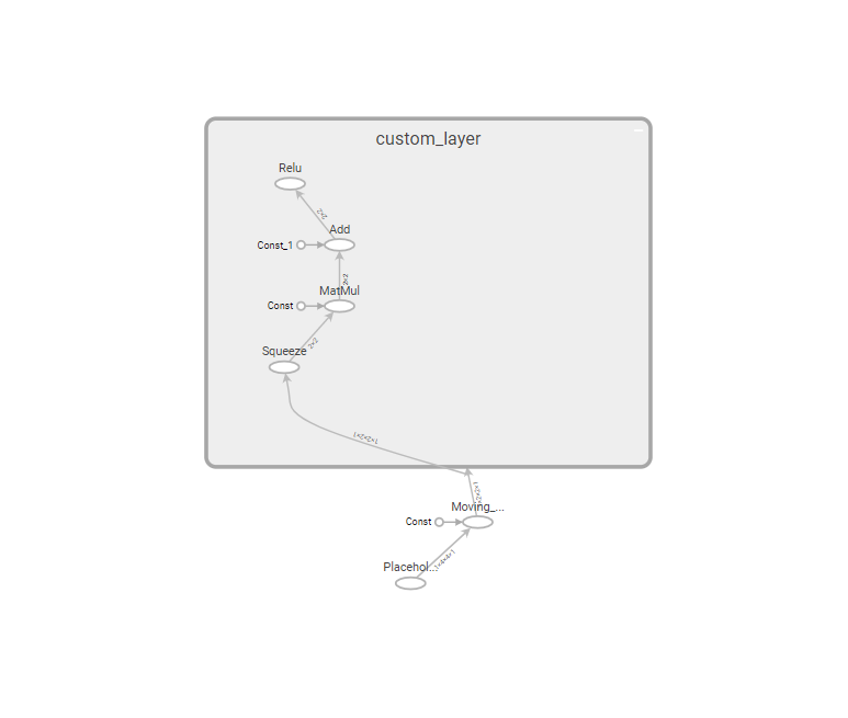
总结:这一次,一开始主要讲了矩阵的一些操作,后续又进行了数学操作,激活函数,运算图、层内元素嵌套运算还有最好的多层运算,并给出了tensorboard的计算图结构。大家不仅仅要看一看,也要动手做一做哦。

一如既往的有什么问题可以直接联系milittle,air@weaf.top邮箱